Solar System — an astronomer’s guide to Living Observatory
Explore JPL-based orbits, planetary maps, Voyager and three scenario labs. A practical guide to the data, scale and scientific limits behind the demo, with eight original screenshots.
Open Solar System — Living Observatory
How does the Solar System look when distances remain linear, planetary sizes are honest, and the date can move in either direction? Living Observatory is an interactive 3D environment for exploring those questions. It combines ephemerides, planetary imagery, moons, spacecraft and educational experiments in a browser. For an astronomy enthusiast, its most useful feature is the connection between a visible object, its numerical state and the provenance of that state.
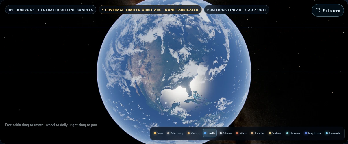
The cover shows Earth in the demo. All eight images in this article are actual application screenshots, captured for this guide; they are not telescope observations. The interface labels below follow the demo’s English controls.
1. Read the Solar System as data
In the normal observatory, motion comes from bundled JPL Horizons ephemerides. The browser interpolates sampled positions and velocities with cubic Hermite interpolation. It is reading a precomputed description of motion, rather than solving a new many-body problem whenever you press Run.
The main planetary bundle covers 2000–2100. The clock accepts UTC, converts to the internal TDB time scale, and supports pause, reverse and accelerated playback. Positions are geometric, expressed in the project’s J2000 ecliptic reference frame. This is a spatial explorer, not an apparent, topocentric sky chart for telescope pointing: light-time, an observer’s horizon and atmospheric refraction are not the displayed coordinate model.
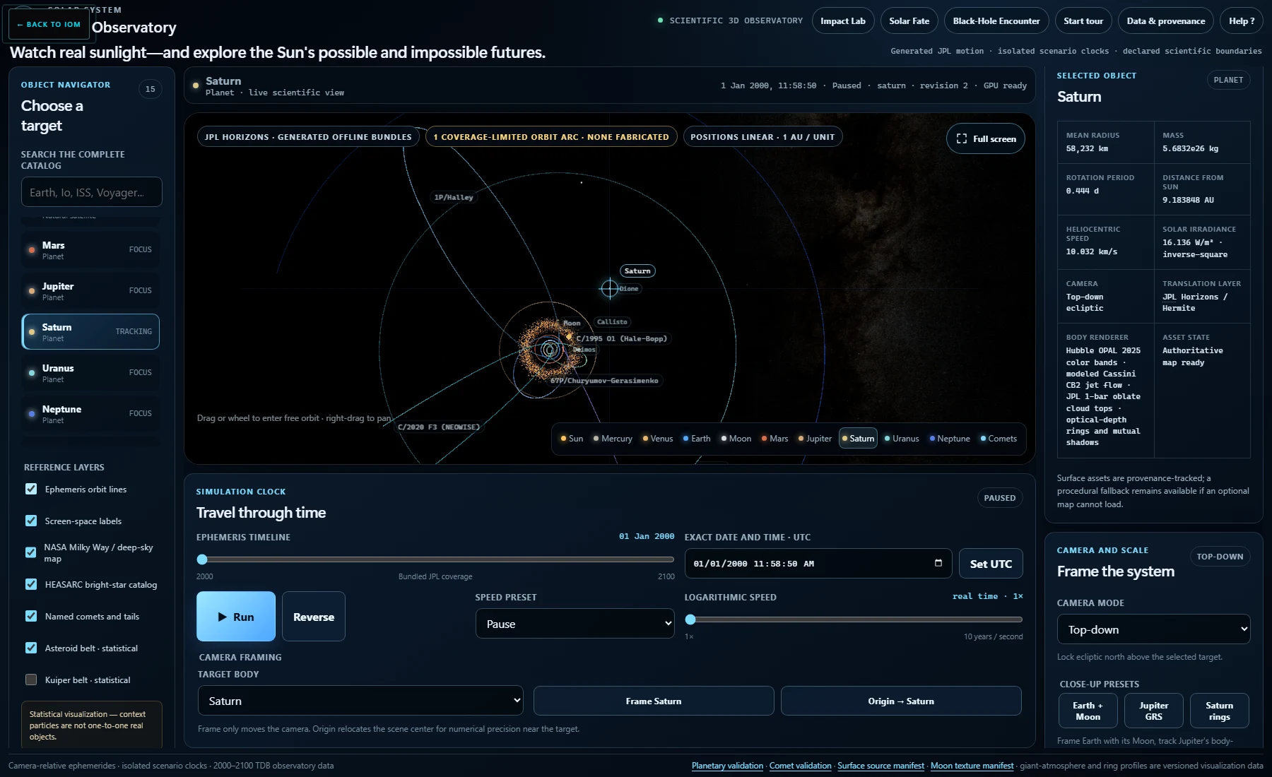
Select a body to inspect its radius, mass, rotation period, distance from the Sun, heliocentric speed and solar irradiance. These readouts make useful comparisons possible: watch speed vary along an orbit or compare the inverse-square decline in sunlight between Earth and the outer planets.
2. Scale, orbits and the camera
True scale is the starting mode. Distances are linear, with one scene unit representing one astronomical unit; physical radii are correspondingly small. At a system-wide distance, labels and selection markers help locate objects that may be smaller than a pixel. They do not represent a planet’s physical diameter.
Presentation enlarges bodies for readability while retaining orbital positions. Compare both modes before judging separations from a screenshot. Orbit lines follow ephemeris samples, rather than a collection of ideal ellipses. A century of data does not contain Neptune’s complete roughly 165-year revolution, so its coverage warning matters. Spacecraft and individual catalog objects can have different time windows.
Use the navigator to focus a body, drag to orbit and scroll to zoom. Camera modes include a top-down ecliptic view, body follow and velocity chase; close-up presets frame Earth with the Moon, Jupiter’s Great Red Spot and Saturn’s rings. Changing the camera changes the view, not the underlying distance scale.
3. Planetary surfaces are maps with a history
Earth combines mapped land and ocean, clouds and night lights with atmospheric scattering. Mars uses Viking colour imagery and MOLA-derived normal detail. Jupiter and Saturn draw on dated imagery, including Hubble OPAL products. Saturn’s rings add radial structure, divisions and planet–ring shadows. Normal detail suggests relief through lighting; it is not resolved, displaced terrain everywhere.
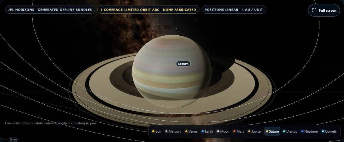
A date on the simulation clock does not turn these maps into historical weather. Cloud composites, surface mosaics and storm details have their own acquisition dates. Uranus and Neptune use authored procedural cloud tops with restrained visible-light colours, not measured global weather maps. Their subtle appearance should not be confused with the strong contrasts of processed infrared images. The Sun similarly combines procedural photosphere and corona effects with dated solar-image detail; it is not a live solar feed.
Open Data & provenance to inspect source attribution and model boundaries. That distinction is essential when using a beautiful close-up to explain real astronomy.
4. Moons, comets and spacecraft
The searchable catalogs extend beyond the eight planets. They include natural satellites, Earth satellites, named comets and interplanetary probes. Catalog membership, a rendered detailed body and available ephemeris coverage are separate things; a catalog entry should not be read as a claim that every moon has an observed surface map.
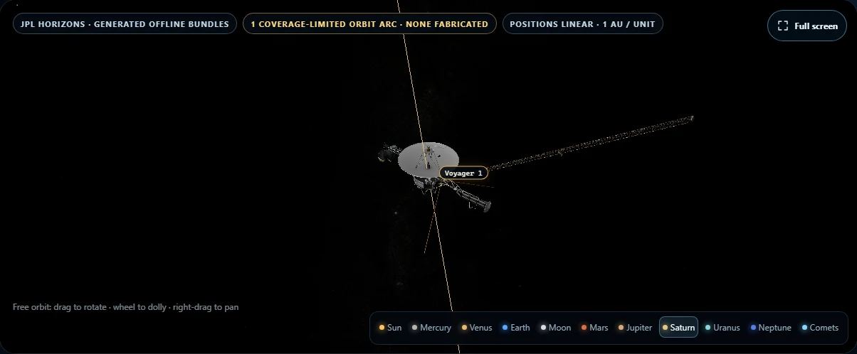
Voyager 1 and 2 use a detailed NASA spacecraft model that can be inspected by zooming in and out. Their trajectory lines refer to position data; the displayed antenna orientation is illustrative, not an attitude-telemetry reconstruction. Earth-satellite motion uses bundled OMM elements with SGP4/SDP4 propagation within the application’s declared validity window, rather than a live tracking feed.
The five named comets include Halley, Encke, 67P, Hale–Bopp and NEOWISE. An ion tail points away from the Sun, while the dust tail curves through an illustrative emission history. These effects explain geometry, not a measured forecast of comet activity. Likewise, asteroid-belt and Kuiper-belt particles are statistical context, not individually tracked minor planets. The background sky provides visual context rather than a date-dependent astrometric star field.
5. Impact Lab: compare causes and outcomes
Impact Lab isolates an event from the observatory clock. Choose the target, impactor diameter, density, speed, entry angle, direction and location; then examine atmospheric entry, fragmentation or airburst, and surface effects. Earth distinguishes land from ocean, with simplified crater, plume, water-cavity and wave behaviour.
A useful experiment is to change one parameter at a time. For the same density, doubling a spherical impactor’s diameter multiplies its initial mass by eight. Doubling its speed multiplies its initial kinetic energy by four: E = ½mv². Atmospheric losses and fragmentation mean that initial energy and energy delivered to the surface are not interchangeable.
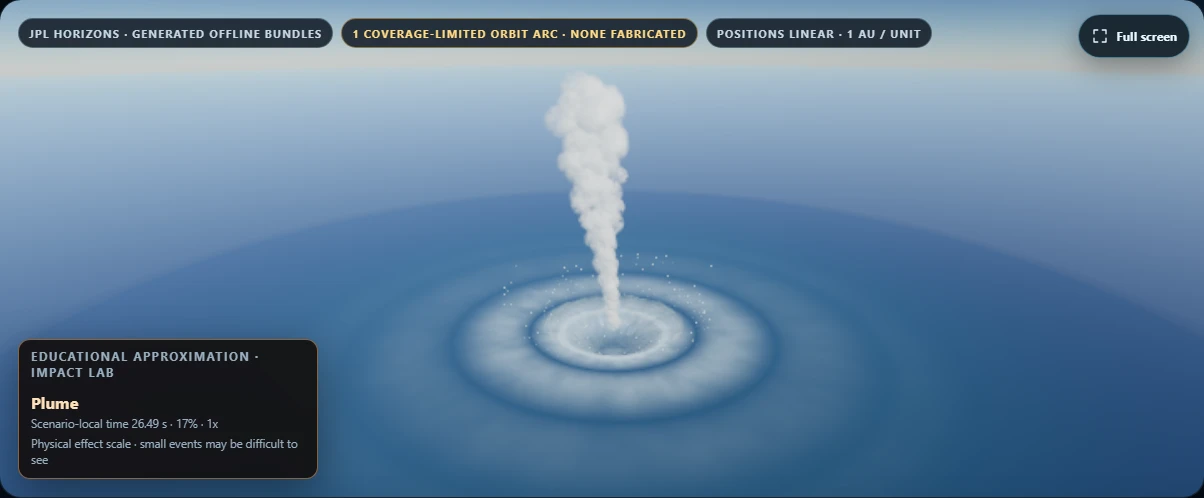
Compare the physical readouts with the visibility setting: enlarging a rendered effect does not enlarge the reported event. This is not a planetary-defence assessment, a casualty model or a tsunami forecast. Pause, replay and reset make it useful for discussing mechanisms and sensitivity without presenting those simplifications as predictions.
6. Solar Fate: the Sun’s future, with the categories kept clear
The scientific evolution sequence compresses stages into an explorable presentation: the present Sun, red-giant expansion, heating of the inner system, loss of outer layers, and a white dwarf that cools. Stage navigation and camera choices let you compare the star itself with the scale of the surrounding material.
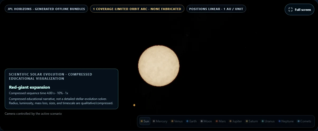
This is an illustrated evolutionary sequence, not a stellar-structure calculation. Times, size changes and transitions are simplified; it does not settle Earth’s eventual survival or compute the future orbits of all planets. The astrophysical distinction is fundamental: the Sun is not massive enough to end as a core-collapse supernova.
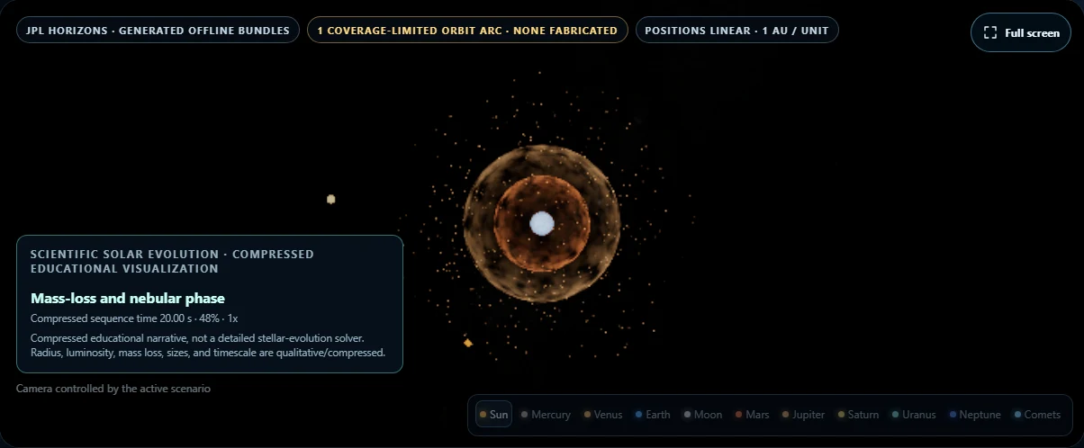
The separate Fictional Solar Supernova option is explicitly impossible for our Sun. It is a cinematic experiment, and should remain labelled as such when sharing images or using the demo in a presentation.
7. Black-Hole Encounter: gravity versus cinematic capture
Physics Flyby copies the current Sun, Moon and planetary states into a separate Newtonian N-body simulation. Initial position, velocity and mass can lead to different outcomes; capture is not guaranteed. Numerical diagnostics help inspect the experiment, but do not provide a research-grade uncertainty estimate.
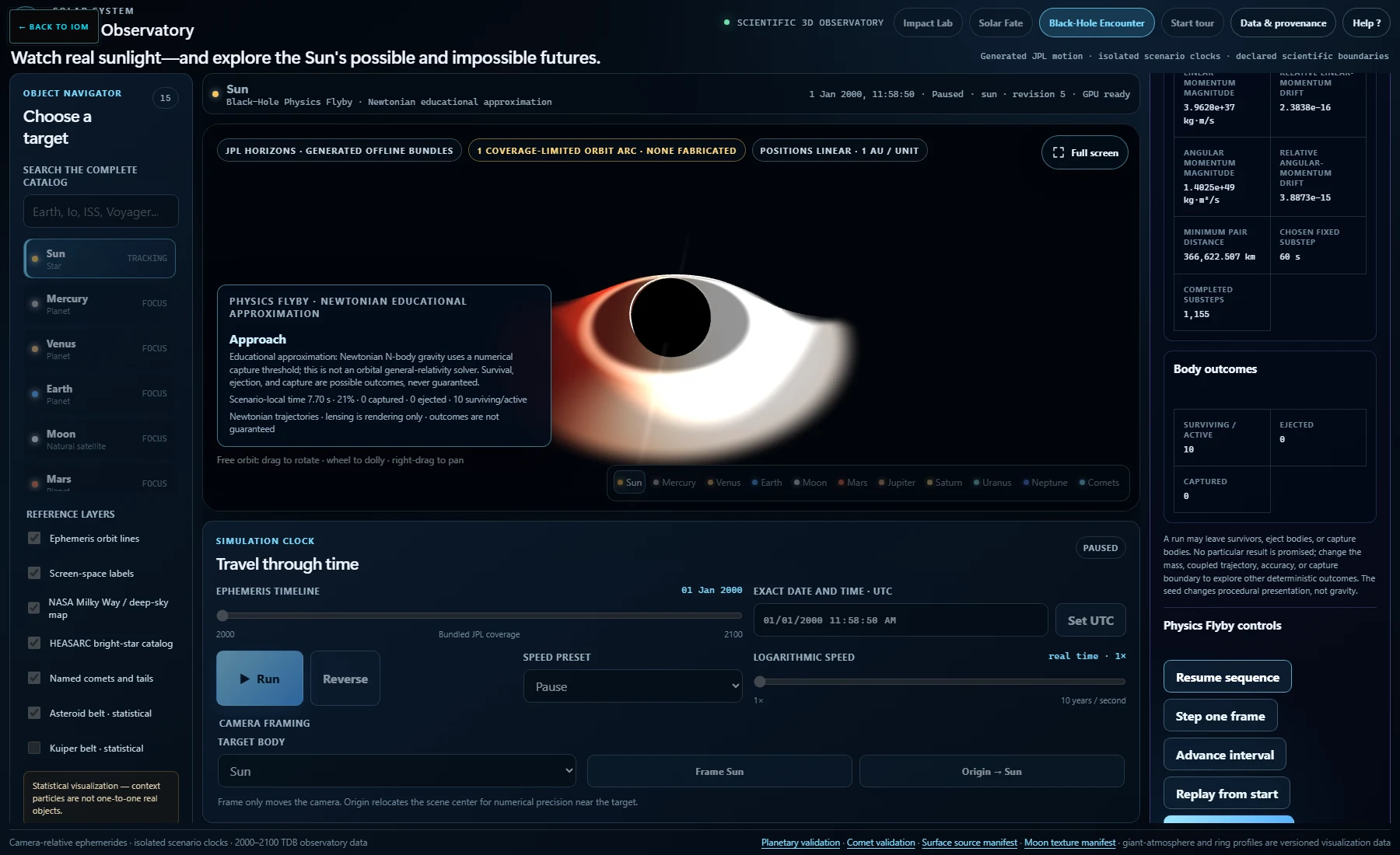
The model is not a general-relativistic or hydrodynamic calculation. Its visual lensing does not feed back into the trajectory integrator. The separate Complete Consumption — Cinematic mode deliberately adds artificial damping to force infall. A black hole does not automatically vacuum up distant planets merely because it is a black hole: mass, distance and the initial orbital state still matter.
8. A useful first observing session
- Start with Earth and the Moon in True scale, then compare Presentation. Notice how much a radius change alters your impression of empty space.
- Choose an outer planet, inspect its coverage notice and reverse the clock. Distinguish an incomplete data arc from an orbital anomaly.
- Focus Voyager, zoom toward the model and back toward its path. Read the source and time window before interpreting its position.
- Run two Impact Lab experiments differing in one input, then compare the numerical results.
- Explore Solar Fate’s scientific stages before opening its fictional alternative.
A desktop browser gives the controls and graphics more room. Lower visual quality if needed; visual detail and the ephemeris data are separate concerns. Scenarios have their own clocks and reset back to the observatory. The best use of the demo is to move repeatedly between the image, the numbers and the stated assumptions.
Sources and further reading
- JPL Horizons manual: reference systems, time scales and the distinction between geometric and apparent quantities.
- NASA: types of stars: the evolutionary context for red giants, white dwarfs and supernovae.
- University of Oxford: the colours of Uranus and Neptune: why familiar processed images can mislead colour comparisons.
- Data & provenance inside the demo: the sources and limitations of this particular implementation.
Screenshots: IOM, captured from the published demo on 27 September 2026. Underlying imagery and model sources retain the credits listed in the demo. This guide describes that version; bundled data and visual models may change with later releases.